A Walk-through of RiboPy CLI
Introduction 
Ribosome Profiling is a sequencing based method to study protein synthesis transcriptome-wide. Actively translating mRNAs are engaged with ribosomes and protein synthesis rates can be approximated by the number of ribosomes that are translating a given mRNA. Ribosome profiling employs an RNase digestion step to recover fragments of RNA protected by ribosomes which are called Ribosome Protected Footprints (RPFs).
Ribosome profiling data analyses involve several quantifications for each transcript. Specifically, the lengths of the RPFs provide valuable biological information (see, for example, Lareau et al. and Wu et al.). To facilitate ribosome profiling data analyses as a function of RPF length in a highly efficient manner, we implemented a new data format, called ribo. Files in ribo format are called .ribo files.
RiboPy package is an Python interface for .ribo files. The package offers a suite of reading functions for .ribo files, and provides plotting functions that are most often employed in ribosome profiling analyses. Using RiboPy, one can import .ribo files into the Python environment, read ribosome profiling data into pandas data frames and generate essential plots in a few lines of Python code.
This document is structured into several sections. First, we give an overview of the Ribo File format and define transcript regions. Second, we provide instructions and requirements for the installation of RiboPy. Third, we describe how to import a .ribo file to the Python environment and demonstrate essential ribosome profiling data analyses in three sections:
In the "Optional Data" section, we explain the three optional types of data, which may exist in a .ribo file.
- Metadata: A .ribo file may contain metadata for each experiment and for the .ribo file itself.
- Coverage: A .ribo file can keep the nucleotide level transcriptome coverage.
- RNA-Seq: A ribosome profiling experiment can be paired with an RNA-Seq experiment to study ribosome occupancy together with transcript abundance.
In the last section, we describe some advanced features including generating ribo files and getting region boundaries that define transcript regions.
.ribo File Format 
.ribo files are built on an HDF5 architecture and has a predefined internal structure (Figure 1). For a more detailed explanation of the ribo format, we refer to the readthedocs page of ribo.

While many features are required in .ribo files, quantification from paired RNA-Seq data and nucleotide-level coverage are optional.
Transcript Regions
The main protein coding region of a transcript is called the coding sequence (CDS). Its boundaries are called transcription start / stop sites. The region consisting of the nucleotides, between the 5’ end of the transcript and the start site, not translated to protein, is called 5’ untranslated region (5’UTR). Similarly, the region having the nucleotides between the stop site and the 3’ end of the transcript, is called 3’ untranslated region (3’UTR). To avoid strings and variable names starting with a number and containing an apostrophe character, we use the names UTR5 and UTR3 instead of 5’UTR and 3’UTR respectively.
Installation 
RiboPy requires Python version 3.6 or higher.
Availability
The source code of RiboPy package is available in a public Github repository.
Pip
RiboPy can be install via pip:
pip install ribopyConda
It is recommended to install RiboPy in a separate conda environment. For this, install conda first by following the instructions here.
The following commands will download an environment file, called enviroenment.yaml, and install RiboPy inside a conda environmen named ribo.
wget https://github.com/ribosomeprofiling/riboflow/blob/master/environment.yaml
conda env create -f environment.yml
From the Source Code
pip install git+https://github.com/ribosomeprofiling/ribopy.gitGetting Started 
First, we download a sample ribo file.
! wget https://github.com/ribosomeprofiling/ribo_manuscript_supplemental/raw/master/sidrauski_et_al/ribo/without_coverage/all.ribo
Let's see the available commands in ribopy and make sure that it is installed.
! ribopy --help
We can see the documentation for each command using the --help argument. For example:
! ribopy plot --help
! ribopy plot lengthdist --help
We can inquire about the contents of the .ribo file by calling the info command.
! ribopy info all.ribo
The above output provides information about the individual experiments that are contained in the given ribo object. In addition, this output displays some of the parameters, that were used in generating the .ribo file, such as left span, right span and metagene radius.
For a detailed explanation of the contents of this output, we refer to the online documentation of the ribo format.
In what follows, we demonstrate a typical exploration of ribosome profiling data. We start with the length distribution of RPFs.
Length Distribution 
Several experimental decisions including the choice of RNase can have a significant impact on the RPF length distribution. In addition, this information is generally informative about the quality of the ribosome profiling data.
We use the command plot to generate the distribution of the reads mapping to a specific region. This method has also a boolean argument called normalize. When normalize is False, the y-axis displays the total number of reads mapping to the specified region. When fraction is True, the y-axis displays the quotient of the same number as above divided by the total number of reads reported in the experiment.
The following command saves the length distribution plot of the RPFs mapping to the coding region in a pdf file.
Note that the help page of ribopy plot lengthdist tells us that the last arguments must be experiment names.
! ribopy plot lengthdist -r CDS -o length_dist.pdf all.ribo GSM1606107 GSM1606108
! ls length_dist.pdf
Metagene Analysis 
A common quality control step in ribosome profiling analyses is the inspection of the pileup of sequencing reads with respect to the start and stop site of annotated coding regions. Given that ribosomes are predominantly translating annotated coding regions, these plots are informative about the enrichment at the boundaries of coding regions and also provide information regarding the periodicity of aligned sequencing reads. This type of plot is called a metagene plot as the reads are aggregated around translation start and stop sites across all transcripts.
The parameter “metagene radius” is the number of nucleotides surrounding the start/stop site and hence defines the region of analysis. For each position, read counts are aggregated across transcripts. This cumulative read coverage (y-axis) is plotted as a function of the position relative to the start/stop site (x-axis).
We can plot the ribosome occupancy around the start or stop sites using the command plot metagene. The following command produces a pdf file conatining the metagene plot at the stop site for the experiments GSM1606107 and GSM1606108. The values on the y-axis are the raw read counts.
! ribopy plot metagene -s stop \
                       -o metagene_stop.pdf \
                       --lowerlength 15 --upperlength 40 \
                       all.ribo \
                       GSM1606107 GSM1606108
To better compare these experiments, we can normalize the coverage by --normalize.
! ribopy plot metagene -s stop \
                       -o metagene_stop_normalized.pdf \
                       --lowerlength 15 --upperlength 40 \
                       --normalize \
                       all.ribo \
                       GSM1606107 GSM1606108
Users can get the data generating the above graphs by using the --dump argument. The command below stores the metagene coverage, generating the plot, in the file metagene_stop.csv.
! ribopy plot metagene -s stop \
                       -o metagene_stop.pdf \
                       --lowerlength 15 --upperlength 40 \
                       --dump metagene_stop.csv \
                       all.ribo \
                       GSM1606107 GSM1606108
One can simply get the metagene data using the command ribopy dump
! ribopy dump metagene -o metagene_dump.csv \
                       -s stop \
                       --lowerlength 15 --upperlength 40 \
                       all.ribo
To get the metagene data for each transcript, we provide --nosumtrans parameter. We can also sum the results accross the given range of RPF lengths by providing --sumlengths. The following command will take longer than the previous ones because the amount of data being output is substantially larger. Also note that the file extension "gz" will be recognized and the csv file will be compressed in gzip.
! ribopy dump metagene -o metagene_dump_per_transcript.csv.gz \
                       -s stop \
                       --nosumtrans \
                       --sumlengths \
                       --lowerlength 15 --upperlength 40 \
                       all.ribo
A Note on Aggregating the Output 
n the above command, we used two parameters --nosumtrans and --sumlengths. These parameters determine how data is aggregated. More precisely, if --nosumtrans is provided, then the data for each transcript will be included in the output, instead of aggregating data accros the transcripts. If --sumlengths is provided, the data will be aggregated accros a given range of lengths.
Region Counts 
Another important aspect of ribosome profiling data is the number of reads mapping to the different regions of the transcripts, namely, 5’UTR, CDS and 3’UTR. A large number of reads mapping to UTR5 or UTR3 regions might indicate a poor quality ribosome profiling data since ribosomes occupy CDS. Furthermore, the distribution of reads across these regions can be associated with the RNase choice in the experiment. For example in Miettinen and Bjorklund, it was shown that ribosome profiling experiments are dependent on digestion conditions.
Before going into the commands, we briefly explain how region counts are computed, introduce our naming convention and define the regions used in ribo format.
For each read mapped to the transcriptome, we take the first nucleotide on the 5’ end of the read and determine the corresponding region. After doing this for all reads, the accumulated values give us the region counts.
As mentioned earlier, a messenger RNA transcript is partitioned into three regions: 5’UTR, CDS and 3’UTR. For technical reasons, we rename 5’UTR as UTR5 and 3’UTR as UTR3.
It is well-known that ribosomes pause, or move slower, around start and stop sites. As a result, we observe peaks around start and stop sites in metagene plots. This behavior of ribosome makes it harder to perform certain analyses such as coverage, translation efficiency, periodicity and uniformity analysis with accuracy. To tackle this problem, we introduce two additional regions called UTR5 junction and UTR3 junction, and modify the definition of the regions UTR5, CDS and UTR3 as shown in Figure 2. This way, we keep regions around start and stop sites separate when doing such analyses.
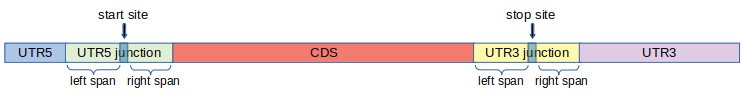
More precisely, first, we fix two integers: left span (l) and right span (r) and define the junction regions as follows.
UTR5 junction: This region consists of l nucleotides to the left of the start site , and r nucleotides to the right of the start site.
UTR3 junction: This region consists of l nucleotides to the left of the stop site , and r nucleotides to the right of the stop site.
Using these junction regions, we re-define the conventional regions as follows.
UTR5: This region is the set of nucleotides between the 5’ end of the transcript and the UTR5 junction.
CDS: This region is the set of nucleotides between the UTR5 junction and UTR3 junction.
UTR3: This region is the set of nucleotides between the UTR3 junction and the 3’ end of the transcript.
The following code will plot the number of sequencing reads whose 5’ ends map to the UTR5, CDS, and UTR3 as a stacked bar plot. To facilitate comparison between experiments, the percentage of the regions counts are plotted and the percentage of reads mapping to CDS are printed on the plot.
! ribopy plot regioncounts -o region_counts_bar.pdf \
                           --lowerlength 15 --upperlength 40 \
                           all.ribo \
                           GSM1606107 GSM1606108
The following command outputs the number of reads, mapping to the coding sequence, summed accros lengths, in a compressed csv file.
! ribopy dump region-counts -o region_counts.csv.gz \
                            -r CDS \
                            --lowerlength 15 --upperlength 40 \
                            --sumlengths \
                            all.ribo
Optional Data 
Length distribution, metagene coverage and region counts are essential to ribosome profiling data analysis and these data exist in every .ribo file. However, for certain types of analysis, additional data might be required. For example, periodicity and uniformity analyses require the knowledge of number of reads at each nucleotide position, aka coverage data. Another analysis, called translation efficiency, can be done when transcript abundance information is present. For these types of analyses, .ribo files offer two types of optional data: coverage data and RNA-Seq data.
It might be helpful to have data explaining how ribosome profiling data is collected, prepared and processed. For this, .ribo files has an additional field, called metadata, to store such data for each experiment and for the .ribo file itself.
Optional data don’t necessarily exist in every .ribo file. Their existence can be checked as follows
! ribopy info all.ribo
In the above output, we see that both of the experiments have all optional data as the values in the columns ‘Coverage’, ‘RNA-Seq’ and ‘Metadata’ are “*”. An absence of “*” would indicate indicate the absence of the corresponding data.
Metadata 
A .ribo file can contain metadata for each individual experiment as well as the ribo file itself. If we want to see the metadata of a given experiment, then we can use the ribopy metadata get command and specify the experiment of interest.
To view the metadata of the .ribo file, we use the ribopy metadata get command without any arguments.
! ribopy metadata get all.ribo
To retrieve metadata from one of the experiments, we provide the parameter --name.
! ribopy metadata get --name GSM1606108 all.ribo
Coverage 
For all quantifications, we first map the sequencing reads to the transcriptome and use the 5’ most nucleotide of each mapped read. Coverage data is the total number of reads whose 5’ends map to each nucleotide position in the transcriptome.
Within a .ribo file, the coverage data, if exists, is typically the largest data set in terms of storage, and it accounts for a substantial portion of a .ribo file’s size, when present. The get_coverage function returns the coverage information for one specific transcript at a time.
Since coverage data is an optional field of .ribo files, it is helpful to keep track of the experiment names with coverage data. Once the list is obtained, the experiments of interest can easily be chosen and extracted.
In the example below, we output the coverage data of the experiment GSM1606108 in a compressed bedgraph file. The coverage data coming from lengths, from 28 to 32 are summed up in the resulting file.
! ribopy dump coverage -o coverage_GSM1606108.bg.gz \
                       --format bg \
                       --lowerlength 28 --upperlength 32 \
                       all.ribo GSM1606108
RNA-Seq 
Most ribosome profiling experiments generate matched RNA-Seq data to enable analyses of translation efficiency. We provide the ability to store RNA-Seq quantification in .ribo files to facilitate these analyses. We store RNA-seq quantifications in a manner that parallel the region counts for the ribosome profiling experiment. Specifically, the RNA-Seq data sets contain information on the relative abundance of each transcript at each of the following transcript regions.
* 5’ Untranslated Region (UTR5)

* 5’ Untranslated Region Junction (UTR5_junction)

* Coding Sequence (CDS)

* 3’ Untranslated Region Junction (UTR3_junction)

* 3’ Untranslated Region (UTR3)
The following command createz a compressed tsv file containing the RNA-Seq data for the experiment GSM1606108 with all the region counts above.
! ribopy rnaseq get --name GSM1606108 \
                    --out rnaseq_GSM1606108.tsv.gz \
                    all.ribo
Advanced Features 
Region Boundaries 
A .ribo file contains the region boundary information. This information can be useful to compare CDS lengths of different transcripts or perform region specific analysis using coverage data.
The following command outputs the region boundaries, in bed format, for the reference used in the ribo file.
! ribopy dump annotation all.ribo > region_boundaries.bed
Transcript Lengths 
The length of each transcript can be obtained, in a tsv file, using the command ribopy dump reference-lengths.
! ribopy dump reference-lengths all.ribo > transcript_lengths.tsv
File Creation 
Using the CLI, .ribo files can be generated from the alignment files. Esentially three files are required.
- Alignment File: In bed or bam format
- Transcript Lengths: In tab separated format
- Region Boundaries: In bed format
Below we give an example of .ribo file creation. First we generate the three input files mentioned above.
TRANSCRIPT_LENGTHS=\
"GAPDH\t20\nVEGFA\t22\nMYC\t17"


TRANSCRIPT_ANNOTATION=\
"""GAPDH    0   5  UTR5    0   +
GAPDH   5  15    CDS 0   +
GAPDH   15  20    UTR3 0   +
VEGFA    0   4  UTR5    0   +
VEGFA   4  16    CDS 0   +
VEGFA   16  22    UTR3 0   +
MYC    0   3  UTR5    0   +
MYC   3  10    CDS 0   +
MYC   10  17    UTR3 0   +"""

READS = \
"""MYC 10  12  len_2_UTR3_junc_1 0   +
MYC 10  12  len_2_UTR3_junc_2 0   +
MYC 0  3  len_3_UTR5_junc_1 0   +
MYC 6  9  len_3_CDS_1 0   +
MYC 10  13  len_3_UTR3_junc_1 0   +
MYC 6  10  len_4_CDS_1 0   +
MYC 6  10  len_4_CDS_2 0   +
MYC 10  14  len_4_UTR3_junc_1 0   +
MYC 10  14  len_4_UTR3_junc_2 0   +
MYC 10  14  len_4_UTR3_junc_3 0   +
MYC 0  5  len_5_UTR5_junc_1 0   +
MYC 10  15  len_UTR3_junc_1 0   +
MYC 10  15  len_UTR3_junc_2 0   +
MYC 10  15  len_UTR3_junc_3 0   +
MYC 10  15  len_UTR3_junc_4 0   +
MYC 10  15  len_UTR3_junc_5 0   +
MYC 10  15  len_UTR3_junc_6 0   +
MYC 10  15  len_UTR3_junc_7 0   +"""

with open("t_lengths.tsv", "w") as t_length_stream, \
     open("t_annotation.bed", "w") as t_annotation_stream, \
     open("reads.bed", "w") as reads_stream:

    print(TRANSCRIPT_LENGTHS,    file = t_length_stream)
    print(TRANSCRIPT_ANNOTATION, file = t_annotation_stream )
    print(READS                , file = reads_stream)
Next, we us the command ribopy create to generate a ribo file named sample.ribo.
! ribopy create -a reads.bed \
                --name sample_exp \
                --reference sample_ref \
                --annotation t_annotation.bed \
                --lengths t_lengths.tsv \
                --radius 2 \
                -l 1 -r 1 \
                --lengthmin 1 --lengthmax 6 \
                sample.ribo
We can easily verify the file creation using the command ribopy info.
! ribopy info sample.ribo
Additionally, one can provide RNA-Seq data or metadata when creating the .ribo files. For details, see the the help page: ribopy create --help.
As another note, when we dump the annotation or the transcript lengths, those files can be used to generate other ribo files. Below we present an example.
! ribopy dump annotation sample.ribo > mock_annot.bed
! ribopy dump reference-lengths sample.ribo > mock_tlen.tsv
! ribopy create -a reads.bed \
                --name sample_exp \
                --reference sample_ref \
                --annotation mock_annot.bed \
                --lengths mock_tlen.tsv \
                --radius 2 \
                -l 1 -r 1 \
                --lengthmin 1 --lengthmax 6 \
                sample_2.ribo
! ribopy info sample_2.ribo